

Robots That See, Part 2: Vision Transformers

Transformer neural nets are quickly making robotics way more useful. See Physical Intelligence’s video they dropped yesterday, where their robot cleans kitchens and bedrooms in homes it was never trained on!
And check out this video from XPENG recapping what they discussed at the ongoing Auto Shanghai show, including how their robot uses more AI chips than their car! Also, watch the end of the video to see their robot working in the car factory!
Video courtesy XPENG.
There’s a lot of semiconductor content in robotics!
If we want to reason about which players are well-suited for the robotics rise, it’s important to understand the fundamentals of how robotics work, and computer vision and transformers are central to today’s robotics revolution.
Wait, what about Intel?
If you read last week’s post, yes, I said we’d cover earnings in this article and take a break from technical topics.
Intel is the obvious company I want to discuss, especially given all the recent news. But Intel reports after the close Thursday, and I’ll be offline Friday driving to my old stomping grounds in Champaign, IL to pace a marathon. So you get this article now, and an Intel article next week.
Fittingly, I’ll be at Intel’s Foundry Direct Connect next week, so I’ll report on Intel earnings and Intel Foundry late next week. Marathon + immediate 6 hour drive home + flight to and from California… I’m gonna be a wreck, but hey, my fingers should still be able to type 😂
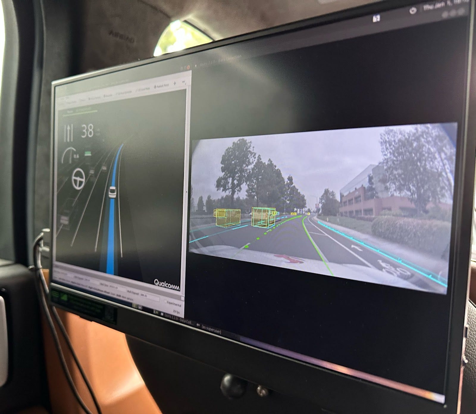
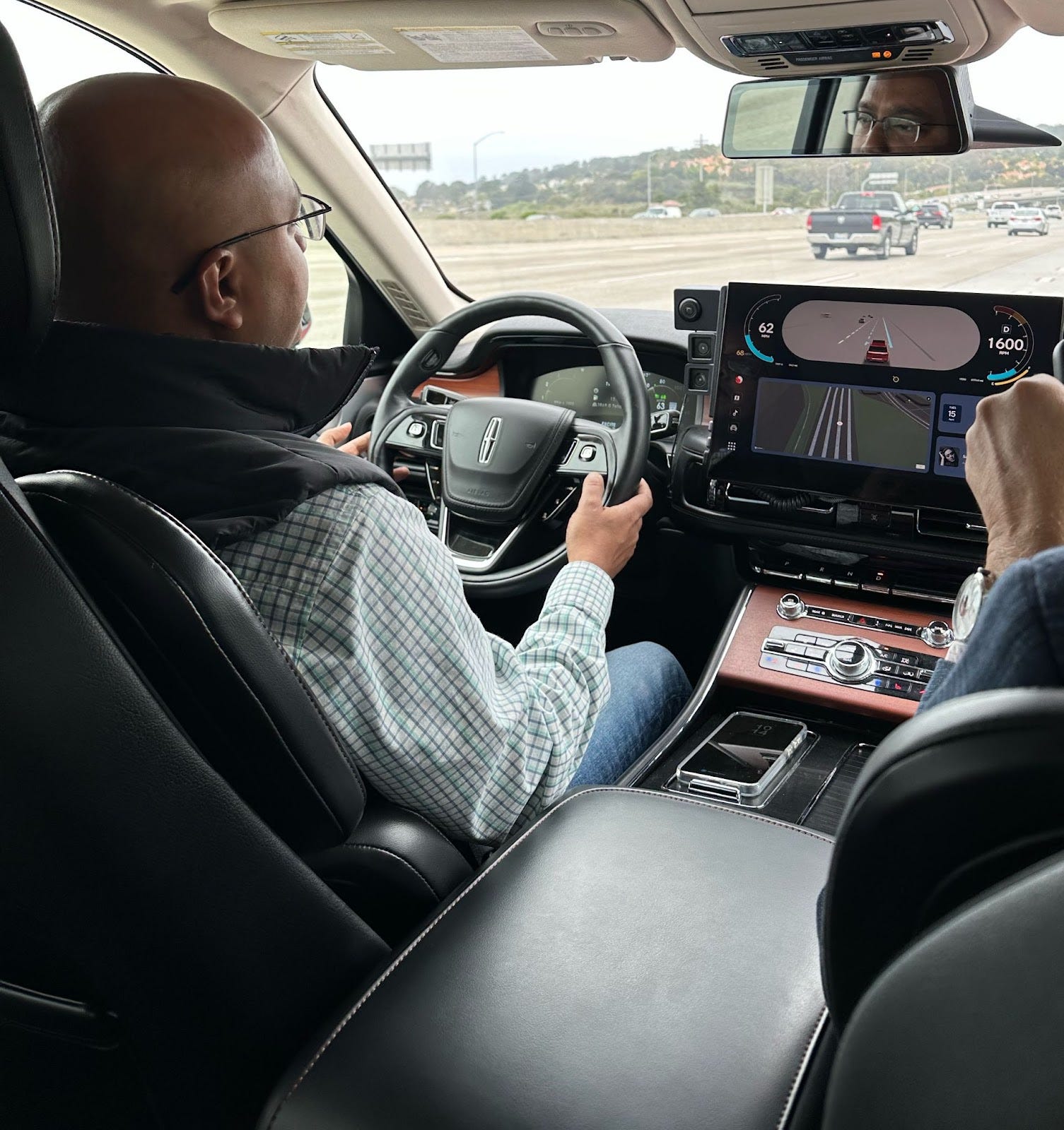
Related to computer vision and traveling: I was at Qualcomm’s Autonomous Driving workshop last week and will share more on that eventually too.
A quick teaser — I went for some Snapdragon powered rides:

Relatedly, I’ve been learning about Intel Automotive as well, which had announcements at Auto Shanghai yesterday:
The second-generation Intel SDV SoC is the automotive industry’s first to leverage a multi-node chiplet architecture, enabling automakers to tailor compute, graphics and AI capabilities to their needs – while reducing development costs and accelerating time-to-market.
Chiplets moving into the automotive industry! The future is disaggregated design!
OK, on with the show.
Vision Transformers
Previously, we examined the history of computer vision with a specific focus on convolutional neural networks. If you missed it:

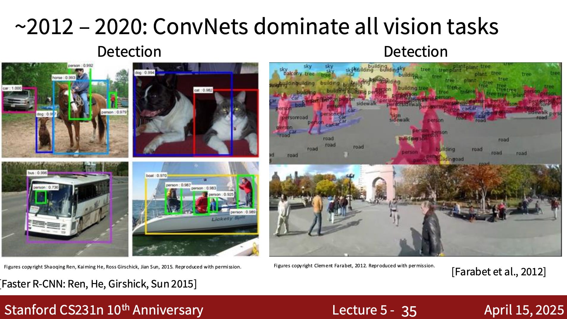
ConvNets took off in computer vision because they’re engineered for image tasks. Their tailored design made them both efficient and broadly useful from 2012 or so onward:
But what happened in 2020?
Well, in 2017 over in language processing land, Google’s Attention Is All You Need paper introduced the Transformer and its self-attention architecture.
Computer vision researchers saw the success of transformers and wondered if they could apply the techniques to vision processing and throw out convolutions entirely.
In late 2020, a different Google team did just that, introducing Vision Transformers. The authors used the same transformer architecture used for text, but with images.
It turns out transformers can match or outperform CNNs for computer vision if trained on sufficiently large datasets!
In this post, we’ll unpack how vision transformers work, why it matters, and the implications for the semiconductor industry.
First, let’s dig into the seminal Vision Transformer paper, also from Google!
AN IMAGE IS WORTH 16X16 WORDS: TRANSFORMERS FOR IMAGE RECOGNITION AT SCALE
The beautiful thing about this paper is that Vision Transformers (ViTs) have a very similar architecture to a language transformer, but simply operate on image “patches” instead of words:

Image patches are just groups of pixels, for example 16x16 square of pixels.
Why operate on patches and not pixels? Self-attention is quadratic, so it doesn’t scale well. Self-attention compares every element to every other element, so for a 224×224 image (~50K pixels), that’s ~50K * ~50K = ~2.5 billion operations.
Instead, we can break the image into say 16×16 patches and only need to do self-attention between these patches. So a 224x224 image has 14x14 patches (196 tokens). Self-attention then only takes 196*196 = ~38K operations, which is much more practical than 2.5 billion operations.
Again, the main takeaway here is image patches as tokens:
Image patches are treated the same way as tokens (words) in an NLP application.
Vision Transformers vs ConvNets
Remember all that talk about how convolutional neural network encode priors into the architecture?
Transformers lack some of the built-in assumptions that make convolutional neural networks so effective for image data. As discussed previously, CNNs have two key inductive biases: locality and translation equivariance. Locality means the model assumes nearby pixels are more relevant to each other than distant ones, and translation equivariance implies that if an object moves slightly in the image the model can still recognize it.
These biases enable CNNs to generalize effectively from limited data.
Transformers, by contrast, treat all input tokens equally and do not assume any spatial structure; self-attention pays attention to all other patches, not just neighbors! ViTs have no inherent preference for local patterns or stability under translation, but have to learn it. This gives them more flexibility, but it also means they need much more data and compute to learn useful visual patterns that CNNs get for free.
Hence seemingly “discouraging” results with smaller training datasets:
When trained on mid-sized datasets such as ImageNet without strong regularization, these models yield modest accuracies of a few percentage points below ResNets of comparable size. This seemingly discouraging outcome may be expected: Transformers lack some of the inductive biases inherent to CNNs, such as translation equivariance and locality, and therefore do not generalize well when trained on insufficient amounts of data.
But the more general Transformer architecture outperforms domain-specific ConvNets when the training set is massive (14M to 300M images)!
Transformers have a more general architecture, yet can learn the priors we humans have encoded into CNNs 🤯
However, the picture changes if the models are trained on larger datasets (14M-300M images). We find that large-scale training trumps inductive bias. Our Vision Transformer (ViT) attains excellent results when pre-trained at sufficient scale and transferred to tasks with fewer datapoints. When pre-trained on the public ImageNet-21k dataset or the in-house JFT-300M dataset, ViT approaches or beats state of the art on multiple image recognition benchmarks.
This is amazing. With enough data, Transformers can learn what ConvNets assume.
And it doesn’t stop there, transformers can go beyond the representational limits of CNNs!
Transformers can learn global dependencies, complex patterns, and relationships that CNNs may miss or struggle to encode efficiently.
How It Works
I’m a big proponent of understanding how things work at a high-level, with most folks needing only enough technical details necessary to appreciate why something matters. The why matters more than the how for most.
But in this case, I think it’s worth diving deeply into how vision transformers work given how important transformers are right now. This will parlay into understanding future innovations like Vision-Language-Action models (VLAs).
So let’s get technical. We’ll zoom back out later (skip ahead if you want).
In model design we follow the original Transformer (Vaswani et al., 2017) as closely as possible. An advantage of this intentionally simple setup is that scalable NLP Transformer architectures – and their efficient implementations – can be used almost out of the box.
Again, the idea is to keep the neural network architecture for image processing as similar as possible to that used in language processing; treating image patches as tokens enables architectural reuse across both vision and language.
Here’s the Vision Transformer architecture (left) and the standard language Transformer (right). Note that the Vision Transformer is simply the standard transformer architecture with some extra pre- and post-processing.

Step 1: Image to Patches
As discussed earlier, the input image is split into fixed-size patches (e.g., 16×16 pixels):

Next, each patch is flattened into a 1D vector, because the standard Transformer receives as input a 1D sequence of token embeddings (e.g., a list of words as the input to an LLM). Since images are two-dimensional, casting them to one dimension is conceptually similar to unrolling all pixel values in a patch into a single line. Flattening makes each image patch look like a “word”, so the ViT can process an image just like it would a sentence.
Say you have a 16×16 patch (256 pixels) from an image. Each pixel has 3 values (RGB), so this patch is a 16×16×3 block. 16×16×3 = 768 values → becomes a 1D vector of length 768. So it’s like reading every RGB value from the top-left corner to the bottom-right and placing them in order into a long list.
To make it simpler to draw, now imagine it’s a patch that’s simply 2x2 pixels:

Flattening this patch results in a 1D vector (i.e. list):

So each flattened patch is a list of RGB values, and thus the image is turned into a list of flattened patches (i.e. [[patch 1], [patch 2], …] )
Step 2: Linear Projection
Next up is linear projection. But what in the world does that mean?

So we’ve got a list of flattened patches, but it’s not a format the Transformer can learn from yet. It’s just a bunch of pixels. Nothing that represents edge, lines, corners, etc:

This is where it gets a bit abstract, hang with me. But we need to transform this into something useful. We need to project these RGB values into embeddings by sending each patch through a trainable neural network layer that maps it into a higher-dimensional space, for example in the paper they used 768, 1024, or 1280 dimensions:

This step builds what we call a latent space (or embeddings), where similar patches end up “close together,” and where the dimensions start to encode visual structure.

I know. Latent space is a tough concept because it’s very abstract. Keep hanging in there, and we’ll unravel this.
Conceptually, it’s a bit easier to learn about latent space in language processing:

For LLMs, a latent space is a compressed representation of language data. It’s a mapping of similar words, phrases, or ideas “close together” in latent space so the model can work efficiently. It’s not raw text, but structure the model builds.

This is what we mean when we say LLMs are a “compressed version of the Internet.” They don’t store the raw Internet text like the Wayback Machine, but rather internalize the patterns from the input data. Trillions of words get distilled into billions of parameters that encode relationships between words, phrases, and ideas.
OK, so back to images. Conceptually, the linear projection of images is similar to token embeddings for language. Linear projection takes raw pixel values and maps them into a space where visual structure can emerge. In this latent space, patches with similar visual patterns cluster closer together, and the dimensions begin to encode features such as edges, textures, or even early hints of objects.
At this point, the model doesn’t know what a “cat” or “tail” is yet. However, once patches are embedded in this space, the Vision Transformer can begin to compare, weigh, and reason about the relationships between regions of the image.
Just like LLMs operate over the compressed geometry of language, Vision Transformers operate over the compressed geometry of visual structure.

Relatedly, there’s a fantastic podcast called Latent Space, for example this was a great interview with co-founder of SF Compute Evan Conrad.
If I didn’t explain that well, apologies! Let me know if you got hung up somewhere and I’ll work to improve it.
Step 3: Add Position Embeddings

At this point, we’ve turned every image patch into a vector that lives in a latent space. Each patch embedding encodes some local visual structure; it may pick up on texture, shading, or a part of an edge.
However, the ViT is currently unaware of the x and y coordinates of this patch; the sequence of patch embeddings is only a collection of vectors, lacking order, position, or spatial structure. So the model doesn’t know if a patch came from the top-left of the image or the bottom-right.
But spatial structure matters in vision. Remember the inductive biases built into CNNs? Locality and translation equivariance enable CNNs to assume that nearby pixels are more important and that objects remain recognizable even when shifted slightly in space. Transformers don’t get that for free, but have to learn it, so the position must somehow be included.
To solve this, Vision Transformers inject position embeddings. Each patch embedding receives a learned vector that is added to it, encoding its location within the original image grid. For example, patch five might be in row 2, column 2, so its position embedding captures that spatial information, providing the model with a basic understanding of the layout.
Now the model can distinguish between patches in the “top-left corner” and “bottom-center” even if the visual content is similar!
These position embeddings are trainable parameters. Just like the patch embeddings, they’re learned during pretraining. Note that, like the patches, the model doesn’t just deal with raw data such as RGB or, in this case, raw (x, y) coordinates, but rather it a learned encoding of position that evolves to reflect what the model finds spatially relevant.
Lastly, the ViT prepends a classification token, often referred to as the CLS token.
In order to stay as close as possible to the original Transformer model, we made use of an additional [class] token, which is taken as image representation. The output of this token is then transformed into a class prediction via a small multi-layer perceptron (MLP) with tanh as non-linearity in the single hidden layer. This design is inherited from the Transformer model for text, and we use it throughout the main paper.
This classification token is a learnable vector that doesn’t come from any patch. Think of it as an empty placeholder that will be filled with the classification at the end of the process, i.e. bird, ball, car, etc.
As the patch embeddings move through the Transformer layers, the CLS token interacts with them through attention. By the end, it collects information from across the whole image. Again, this is the vector the model uses to insert the final classification—bird, ball, car, etc.
But we’re still at just the data pre-processing step with this patch + position embedding + (empty) class embedding. The classification comes later.
So now, after the data preprocessing, the model can start learning relationships between parts; it has information about the visual structure of the patch (patch embedding) and where it is (position embedding).
Step 4: Transformer Encoder

Finally, time for the magic to happen! After flattening the image, embedding each patch, injecting positional context, and prepending the classification token, we now have a sequence of vectors ready to enter the Transformer encoder where the actual learning occurs!
The encoder consists of a repeated stack of blocks. Each block contains the same five components, and the stack depth varies depending on model size. In this paper, ViT-Base utilizes 12 layers, ViT-Large employs 24, and ViT-Huge uses 32.
Each encoder block contains:
Layer Normalization
Multi-Head Self-Attention
A Residual Connection
Feedforward MLP
Another Residual Connection
Let’s walk through what each piece does. If you know about this from LLMs, feel free to skip.
1) Layer Normalization
Layer normalization adjusts each patch embedding so its values have a consistent scale. Without normalization the magnitude of the values in the vector can vary widely between patches. For example, some might have very large numbers, others small, depending on the input image and the learned weights from earlier layers.
This inconsistency can destabilize training and make learning harder. Layer normalization fixes this by centering the values in each vector and scaling them, ensuring that all tokens enter the attention mechanism on roughly the same footing so that the model can focus on learning the structure of the data rather than being distracted by arbitrary differences in scale.
2) Multi-Head Self-Attention (MHSA)
This is the heart of the Transformer. For each token in the sequence, including every patch and the classification token, the model looks at every other token and computes a weighted average of them.
It’s basically asking: Which other parts of the image should I consider for understanding this patch? The paper illustrates this nicely:

Multiple attention heads run in parallel and each one learns to focus on a different aspect of the relationships between patches. One head might learn to detect symmetry, another might track long-range dependencies, and others might focus on contrast or texture across the image.
Attention lets every patch look everywhere. A patch in the top-left corner can directly compare itself to one in the bottom-right, with no need for spatial proximity or hierarchical structure. That is very different from convolution, which moves information locally and incrementally.
This is key in helping ViTs outperform ConvNets!
3) Residual Connection (after attention)
After the attention operation, the model adds the original input back to the attention output. This is called a residual connection. It helps preserve useful features from earlier layers and ensures that gradients can flow backward during training without vanishing or exploding.
Why include the original input? That seems redundant…
Well, not every attention layer improves the representation, so the residual connection allows the model to carry forward what already works.
4) Feedforward Multi-Layer Perceptron (MLP)
Next comes an MLP block, which is a small neural network applied to each patch embedding independently. It typically consists of two layers with a non-linear activation in between, such as RELU or GELU.
For more information, see Grant Sanderson’s language modeling tutorial which helps gives intuition.
Basically, attention by itself is a linear operation, which limits the kinds of patterns it can express. The MLP injects non-linearity and allows the model to detect more complex combinations of features.
I guess the takeaway is that this step helps the model go from just noticing features to understanding their interactions.
5) Another Residual Connection (after MLP)
Just like after the attention block, the output of the MLP is combined with its input through another residual connection. Again, this ensures that the model can preserve useful information and only apply transformations where needed.
Summary
After these five steps, each patch now carries information not only about its own content but also about how it relates to every other patch in the image!
The classification token, having attended to all patches, now holds a summary of the entire image. This sets the stage for the final step: classification.
Step 5: MLP Head and Classification

At this point, the classification token has passed through the full Transformer stack and interacted with every patch in the image to gathered global context. But it doesn’t have a class prediction yet.
ViT passes it through one last module: the MLP head. This is a small feedforward neural network that maps the final classification token to the output space.
The MLP head learns how to interpret the aggregated information in the classification token and translate it into a decision. If the CLS token is the summary of the image, the MLP head serves as the final judge, assigning a label.
Finally, the model outputs a prediction! It’s a bird! It’s a plane! It’s Superman!

For paid subscribers we’ll talk about the results from Vision Transformer paper, and then implications for the semiconductor industry from training and inference hardware to implications for robotics and automotive.