This piece kicks off a new series on robotics. I’ll walk through the key ideas from first principles, starting with computer vision, and explain how GenAI changes what’s possible in robotics.
Note that I'm pulling on some other ongoing threads on Chipstrat, so after this post, we’ll take a break from technical topics and cover earnings season for a bit.
Even though this one gets technical, hang with me as we will cover fun and important computer vision history!
Robotics has long felt like it was almost ready. Kind of like autonomous driving, where each year we kept saying “It’ll be here in just a few years…”
Yet robotics has recently undergone rapid, significant progress. Why?
Generative AI, of course!
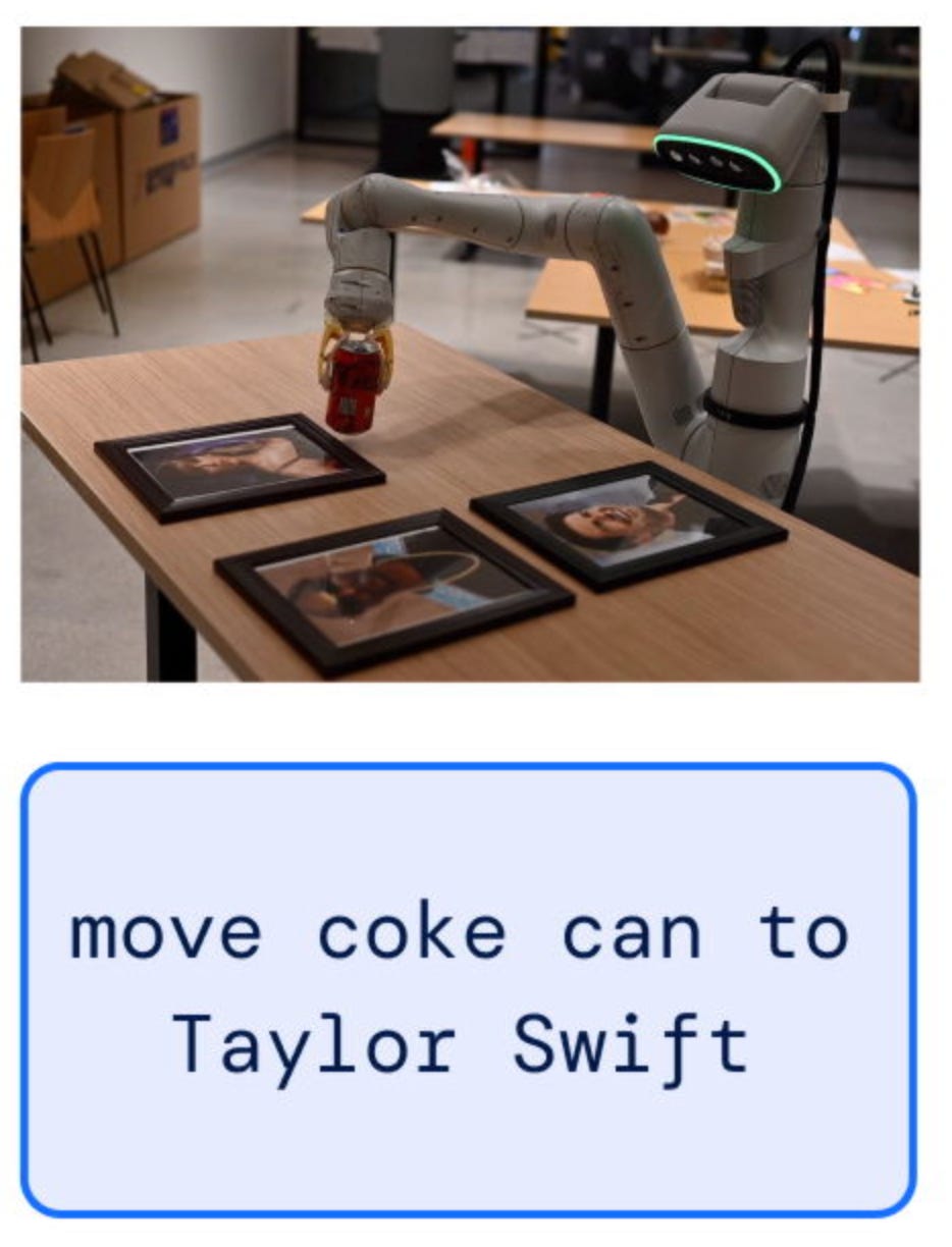
Large vision-language models trained on Internet-scale data dramatically improve robotic generalization. Robots can execute a command like “place the Coke can next to Taylor Swift”:
It’s helpful (and fun) to trace the arc of computer vision from CNNs to transformers to understand how we got here.
We’ll also study the technical stack as we go and compare with today’s tools.
Computer Vision, from CNNs to Transformers
Robots need to see! That means bots need to make sense of images.
Convolutional neural networks have historically played a key role in helping robots interpret visual data.
Convolutional Neural Networks
A convolutional neural network (also called a ConvNet or CNN) is a feed-forward neural network designed for image inputs.
The architecture is specialized for computer vision, encoding domain-specific assumptions (priors) about how images are structured. For example, ConvNets assume that nearby pixels are related and that edges are important. These patterns aren’t learned; they’re embedded in the architecture.
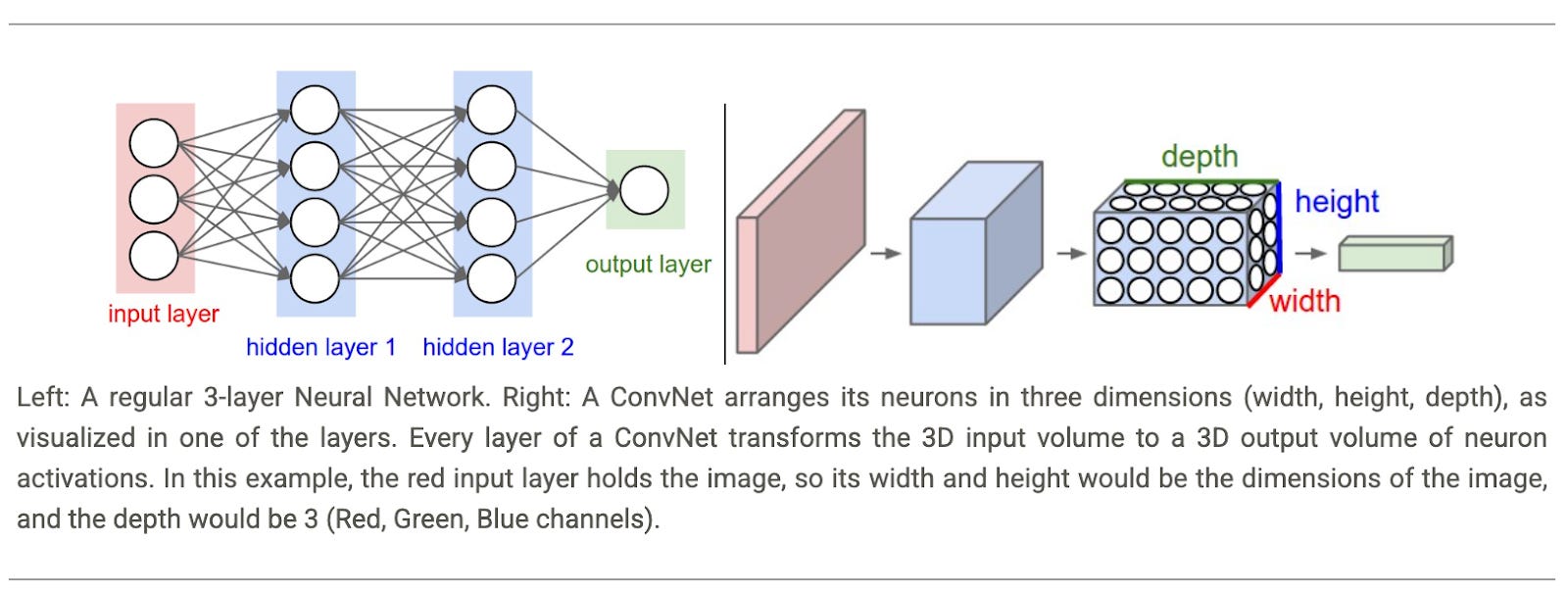
Convolutional Neural Networks take advantage of the fact that the input consists of images and they constrain the architecture in a more sensible way. In particular, unlike a regular Neural Network, the layers of a ConvNet have neurons arranged in 3 dimensions: width, height, depth.
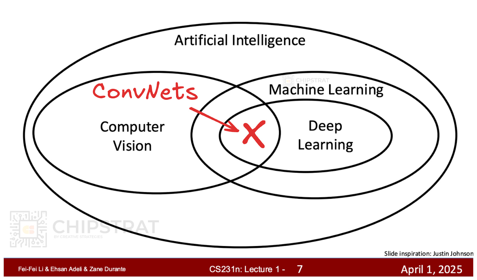
CNNs aren’t generic; they’re a type of specialized neural network architecture. I’m taking the time to point out because it’s important later.
CNNs or ConvNets are a deep learning architecture tailored for computer vision
If, like me, you’re wondering what a “convolution” is — see this video from 3Blue1Brown (Grant Sanderson is the best of YouTube in my opinion!)
CNNs have a rich history full of insights that still matter today. Let’s dig in!
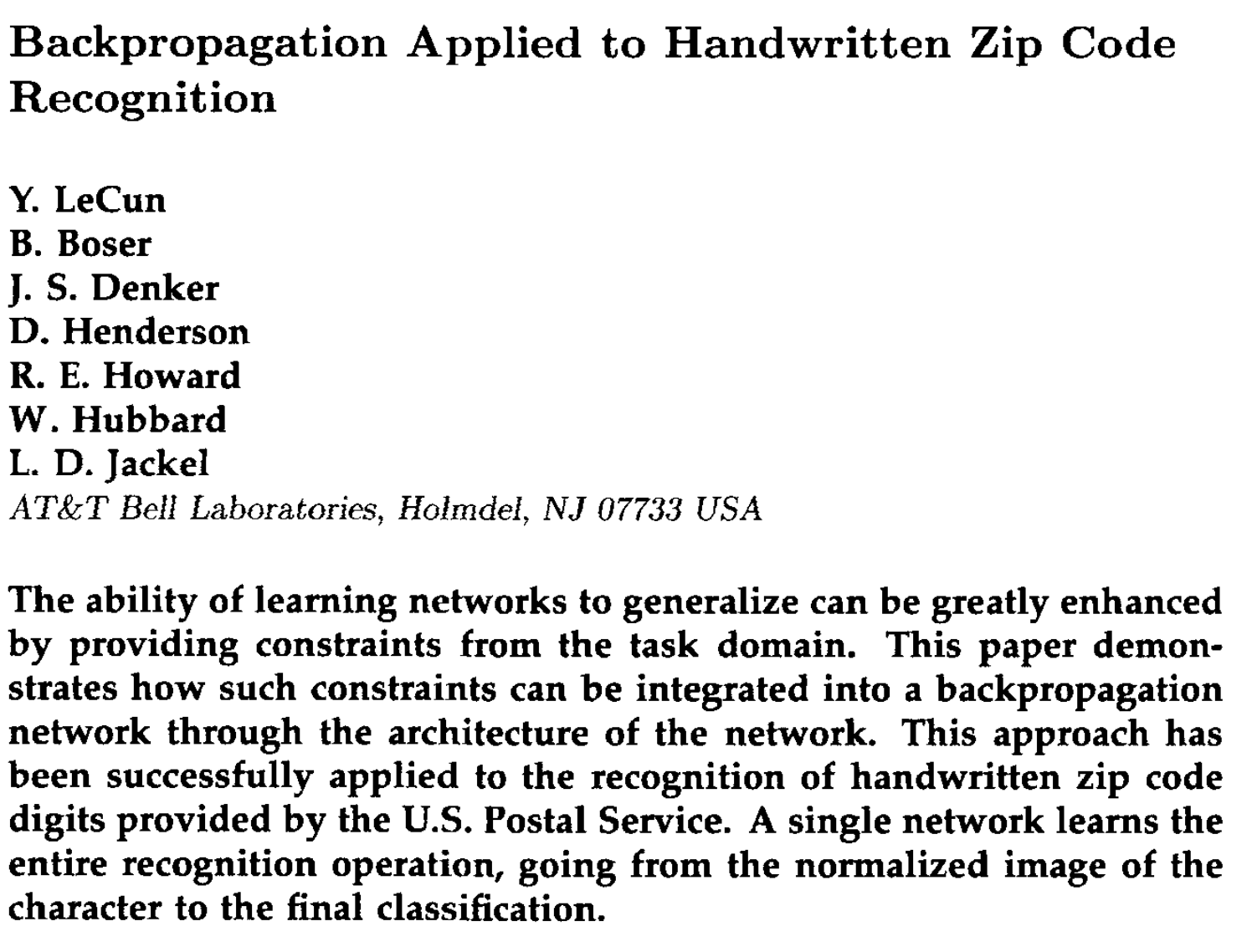
Backpropagation Applied to Handwritten Zip Code Recognition
Notice how this summary paragraph emphasizes the usefulness of providing constraints from the task domain, aka encoding priors.
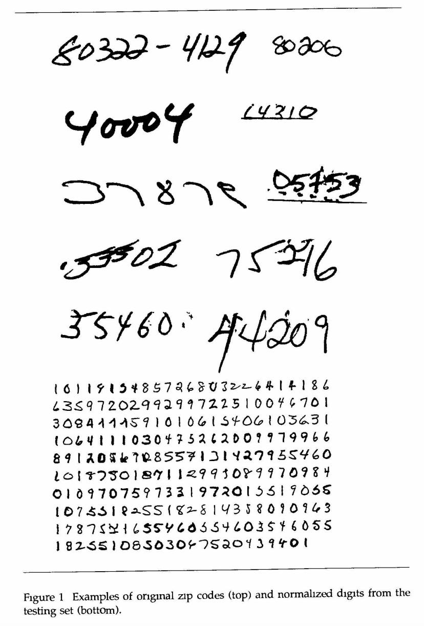
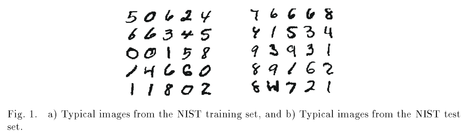
The results in this paper, especially in the context of THIS RESEARCH HAPPENING IN 1989 are fantastically impressive. And incredibly practical and useful too. Look at the variations in handwritten digits in the training data:
The neural network in this paper worked with an incredibly small (by today’s standards) dataset: ~7000 images of digits used to train the model, and ~2000 held back for testing.
The data base used to traın and test the network consists of 9298 segmented numerals digitized from handwritten zip codes that appeared on U.S. mail passing through the Buffalo, NY post office. Examples of such images are shown in Figure 1. The digits were written by many different people, using a great variety of sizes, writing styles, and instruments, with widely varying amounts of care; 7291 examples are used for training the network and 2007 are used for testing the generalization performance.
How quaint! By the way, this data was hard to gather then, and it’s still no easy task.
Locating the zip code on the envelope and seрarating each digit from its neighbors, a very hard task in itself, was performed by Postal Service contractors (Wang and Sriharı 1988).
And the model was small too, only ~1000 neurons and ~70K weights.
Of course, 1989 was long before PyTorch and GPUs! Instead, these Bell Lab researchers used SN, a simulator built in 1988, to train their neural networks. SN was used to implement the full neural network training loop, including forward pass, error backpropagation, and weight updates. The conceptual role of SN in 1989 was similar to what PyTorch or TensorFlow provide today: it encapsulated the mechanics of training so researchers could focus on the model itself.
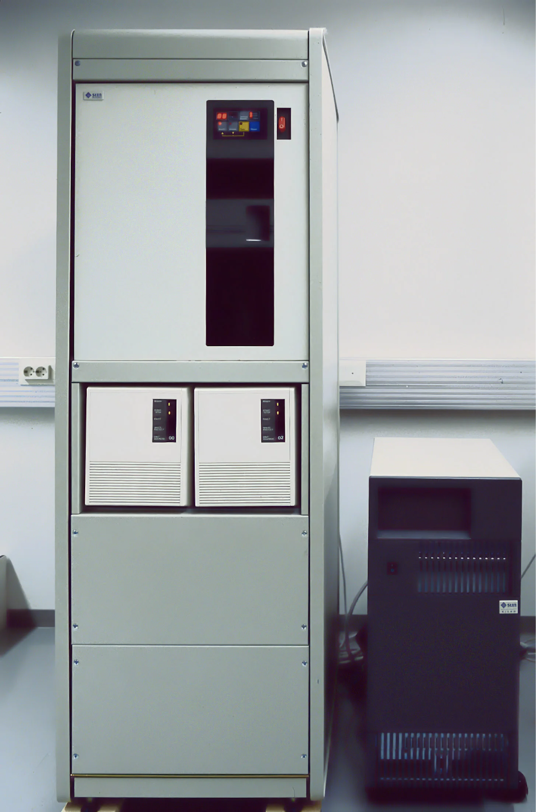
As for hardware, this convolutional neural net was trained on SUN-4/260 workstations:
“This machine had a 16.67 MHz SPARC processor, 64 Mbytes memory, 2 × 1 Gbyte SCSI disks, and a 10 ½ ″ open-reel magnetic tape drive.” Source
Even with the small network size, it took 3 days to train the neural net on this hardware.
YL: Back then, neural nets were hard to use. You had to implement backpropagation in Fortran or C—Python and MATLAB didn’t exist yet. You’d initialize weights poorly, use small networks based on textbook advice, and train on limited data like XOR. It worked inconsistently. Many gave up. You needed a bag of tricks to make it work, and those tricks weren’t well known or documented.
Software platforms didn’t exist yet, so you wrote everything from scratch. We had to build our own Lisp interpreter and hook it into a neural net library. Eventually, around 1991, we invented modular systems where each module knew how to forward- and back-propagate gradients, and we connected them in graphs. We compiled Lisp to C for production systems at Bell Labs.
Lisp and C! Python didn’t even exist yet.
Inference Accelerator
After training the NN in this paper, the model was moved to a digital signal processor (DSP) for inference.
Take note! Back in 1989 Lecunn used what can be thought of as a primitive AI accelerator for inference! The Bell Lab researchers trained on a slower but more general purpose HPC workstation and then ran inference on a fast parallel processing system (DSP) attached to a host PC.
Even in the early days of neural nets, it was clear: training and inference are different beasts. Training neural nets was far more demanding than running them
Now, I’m not saying today’s hardware (e.g. Nvidia’s GPU-based AI systems) aren’t great for both. Rather, I’m hinting at why competitors from AMD to startups all start with inference, as it’s much easier to support from a systems perspective.
We saw that in our GPU networking series last week too, right? Recall how training massive modern neural nets require complicated software parallelism strategies, tons of intra- and inter-node communication, and even innovations like network switches that can help do math and reduce the amount of data being shuttled around.
In this paper we can even see glimpses of using supercomputers for training but edge AI systems for inference. So keep that in the back of your mind.
Anyway, back to 1989:
Little did we know, December 1989 was a monumental month for the world with the birth of computer vision (or at least this milestone paper) and, ya know, Taylor Swift.
The paper tells us a bit more about the inference hardware:
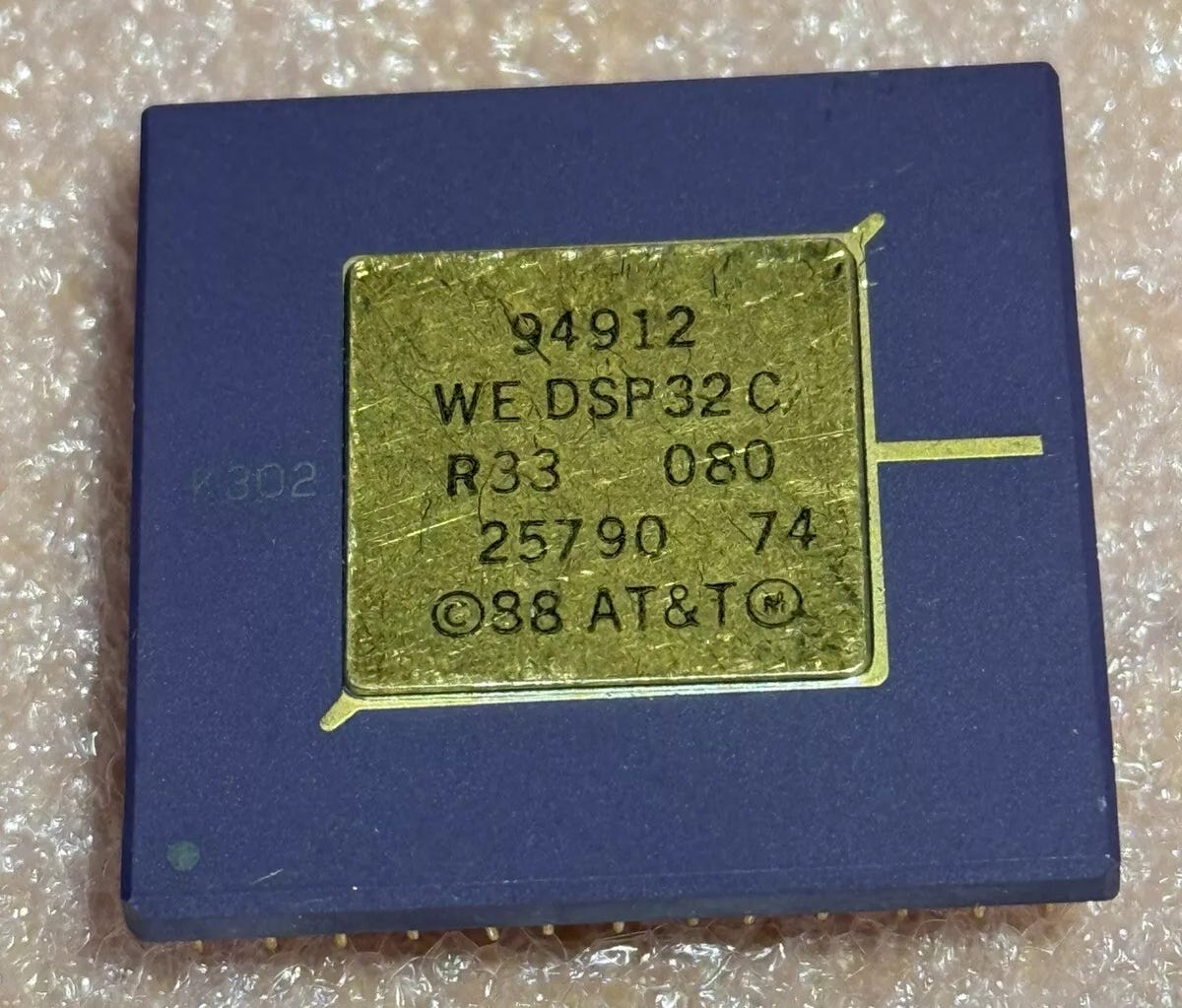
During the recognition process, almost all the computation time is spent performing multiply accumulate operations, a task that digital signal processors (DSP) are specifically designed for. We used an off-the-shelf board that contains 256 kbytes of local memory and an AT&T DSP-32C general purpose DSP with a peak performance of 12.5 million multiply add operations per second on 32 bit floating point numbers (25 MFLOPS). The DSP operates as a coprocessor; the host is a personal computer (PC), which also contains a video acquisition board connected to a camera… On normalized digits, the DSP performs more than 30 classifications per second.
It’s just a bunch of multiply accumulates! We covered that here if you need a refresher.
For perspective, 3 days of training on this DSP (25 MFLOPs of FP32) is equivalent to less than one second of training on an Nvidia H100 (67 TFLOPs for FP32)!
The DAU employs a four-stage pipeline to perform 25 million floating-point computations per second. Configured for multiply/accumulate operations, the DAU is the primary execution unit for signal processing algorithms.It contains a floating point multiplier and a floating-point adder that work in parallel to perform computations of the form a = b + c*d. The DAU has four 40-bit accumulators. It employs a straightforward fetch-multiply-accumulate-store pipeline, which we explain in detail later.
We can think of this DSP as a simple scalar parallel processor. It’s a far cry from a modern hardware with native vector, matrix, or tensor processing. But it’s still interesting to know about and understand, especially because many of today’s edge NPUs evolved from DSPs!
If you’re a tinkerer and want to try it yourself, you can buy this chip for $35 OBO on eBay.
DSPs & NPUs for Neural Network Acceleration
A brief tangent so feel free to skip, but broadly relevant. Digital Signal Processors are still found in many edge NPUs today, since many of these NPUs evolved from DSP IP.
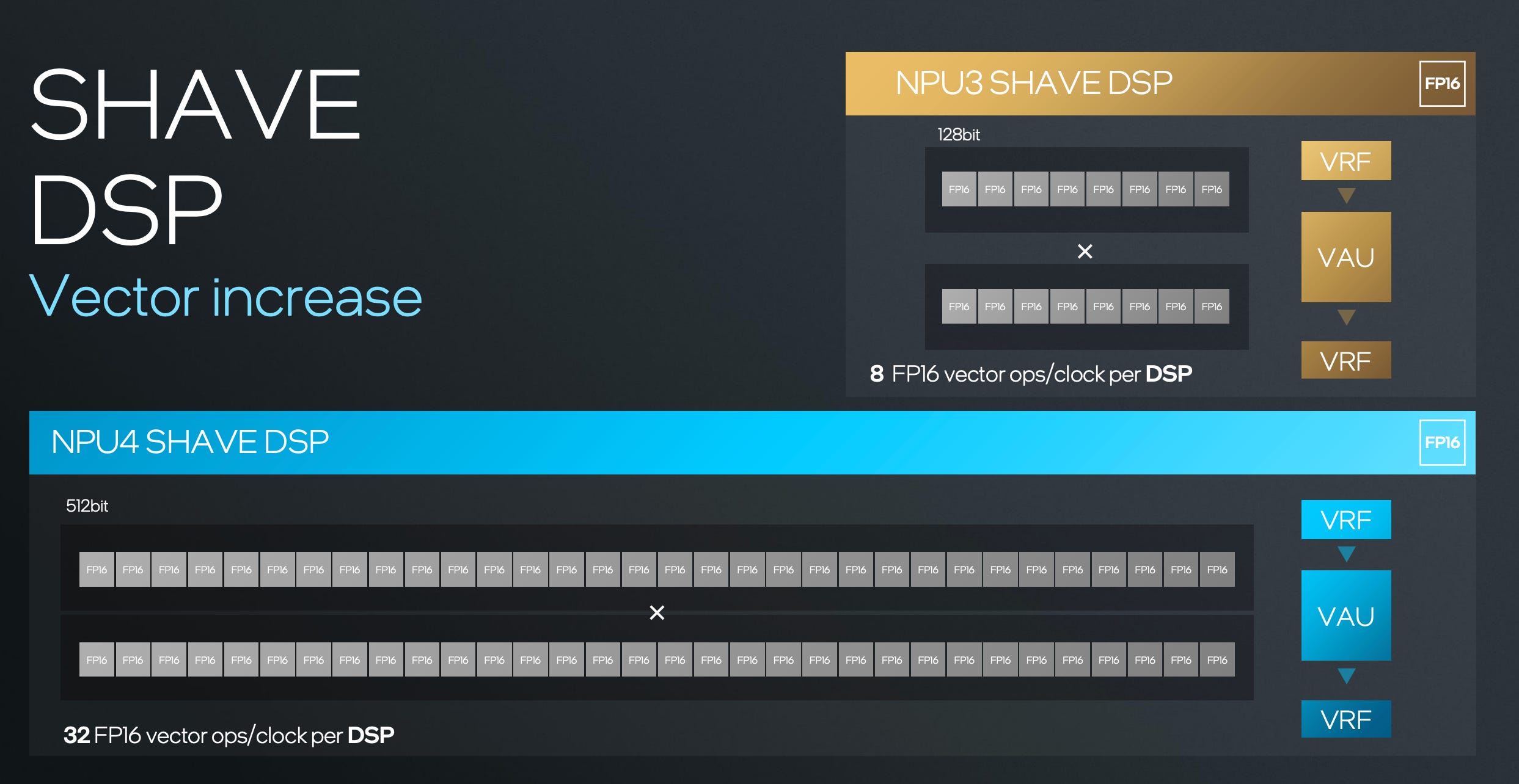
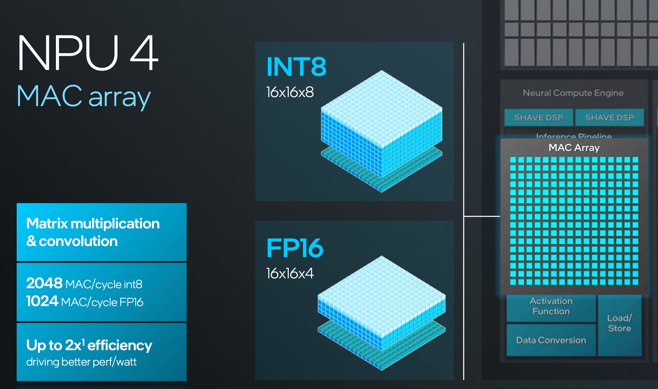
For example Intel’sNPU has a DSP for vector compute and MACs (multiply and accumulate blocks) for matrix math. Lots of info in this video from Intel regarding the Intel NPU architecture and how it runs LLMs:
Intel’s SHAVE (Streaming Hybrid Architecture Vector Engine) DSP focuses on vector computations. This IP was acquired from Movidius.
Intel’s NPU also natively supports matrix computations with its MAC units.
Qualcomm’s NPU has a history dating back to DSP IP as well.
In 2007, the first Hexagon DSP was launched on the Snapdragon Platform — the DSP control and scalar architecture was the basis for our future NPU generations. In 2015, the Snapdragon 820 processor was announced and included our first Qualcomm AI Engine to support imaging, audio, and sensor use cases. We added the tensor accelerator to the Hexagon NPU in the Snapdragon 855 in 2018. The following year, we expanded the use cases for on-device AI on Snapdragon 865 to include AI imaging, AI video, AI speech, and always-on sensing.
In 2020, we achieved a major milestone with a revolutionary architecture update for the Hexagon NPU. We fused together the scalar, vector, and tensor accelerators for better performance and power efficiency. A large-shared memory was dedicated for the accelerators to share and move data efficiently. The fused AI accelerator architecture established a solid foundation for our NPU architecture moving forward.
Qualcomm’s NPUs have been updated to include tensor/matrix support, and they have software innovations too like their “microtile inferencing” which can be thought of as an orchestration algorithm:
Microtile inferencing leverages the Hexagon NPU scalar capacity to break networks into small microtiles that can be executed independently. This eliminates memory traffic between as many as 10 or more layers, maximizes utilization of the scalar, vector, and tensor accelerators within the Hexagon NPU, and minimizes power consumption. Source
Clearly Intel and Qualcomm’s NPUs have architectural and software differences.
So the takeaways of this sidebar here are
Many NPUs evolved from DSPs
No two NPUs are alike.
1989 Learnings
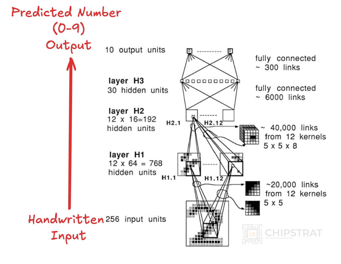
OK, back to Yann LeCun. So the 1989 paper has a nice little diagram to illustrate the neural network architecture, read it from bottom to top:
Let’s break down some of the priors encoded in this ConvNet layer-by-layer:
Input: The input is a 16x16 normalized image. This encodes the prior knowledge that the data is spatially organized in a 2D grid, which is fundamental for image data.
Layer H1: Each unit in H1 takes input from a 5x5 neighborhood in the input image. This enforces the prior that local features are important for image recognition. Moreover, all units within a feature map share the same weights. This is a crucial prior, stating that if a feature is useful in one part of the image, it's likely to be useful in other parts. This is called translation invariance and it allows the network to detect features regardless of their location.
Layer H2: Units in H2 combine local information from H1, called hierarchical feature extraction. This prior suggests that higher-level features can be built from combinations of lower-level features.
Layer H3: This layer combines all the features extracted by the previous convolutional layers. The prior here is that after local and hierarchical feature extraction, the final classification decision should be based on a global combination of all the learned features.
Output Layer: The output uses 10 units, one for each digit class. This is known as place coding, andencodes the prior that the task is a multi-class classification problem where only one digit is present in each image.
These priors, implemented through the convolutional layers, weight sharing, and network architecture, significantly constrain the model and guide it towards efficiently learning useful representations for handwritten digit recognition.
The paper concludes by noting that
This paper shows a useful real-world result
It’s possible on commercial hardware
A key enabler is backpropagation (we didn’t cover much here)
Another key enabler is encoding domain specific priors into the architecture
Software is super important for NN training
These points are bolded in the conclusion below:
We have successfully applied backpropagation learning to a large, real world task. Our results appear to be at the state of the art in digit recognition. Our network was trained on a low-level representation of data that had minimal preprocessing (as opposed to elaborate feature extraction). The network had many connections but relatively few free parameters. The network architecture and the constraints on the weights were designed to incorporate geometric knowledge about the task into the system. Because of the redundant nature of the data and because of the constraints imposed on the network, the learning time was relatively short considering the size of the training set. Scaling properties were far better than one would expect just from extrapolating results of backpropagation on smaller, artificial problems.
The final network of connections and weights obtained by backpropagation learning was readily implementable on commercial digital signal processing hardware. Throughput rates, from camera to classified image, of more than 10 digits per second were obtained.
This work points out the necessity of having flexible "network design'' software tools that ease the design of complex, specialized network architectures.
And for your viewing pleasure, here’s a video demonstrating the usefulness and speed of the final product!
We could stop the article here and I’d be happy — we learned a lot already!
The paper describes the shortcomings of that 1989 database of zip codes, namely that the the dataset contained some noisy / unreadable data, the USPS wouldn’t let them distribute it freely for apples-to-apples comparisons, and the dataset became to small as models improved.
We acquired a database of 7064 training and 2007 test digits that were clipped from images of handwritten Zipcodes. The digits were machine segmented from the Zipcode string by an automatic algorithm. As always, the segmented characters sometimes included extraneous ink and sometimes omitted critical fragments. These segmentation errors often resulted in characters that were unrecognizable or appeared mislabeled. (For example, a vertical fragment of a "7" would appear as a mislabeled "1".) These butchered characters comprised about 2% of test set, and limited the attainable accuracy. We could improve the accuracy of our recognizers by removing the worst o enders from the training set, but in order to maintain objectivity, we kept the butchered characters in our test set.
These “butchered” (lol) characters would ultimately limit the effectiveness of the dataset as CNNs became very proficient at identifying the numbers. If my model is 98.1% accurate and yours is 98.5%, but the test set has 2% untrustworthy data… what to make of whether my model or yours is better? And are we overfitting?
The US Postal Service requested that we not distribute this database ourselves and instead, the USPS, through Arthur D. Little, Inc., supplied other researchers with the unsegmented Zipcodes from which our database was derived. Segmenting was done by the users, often by hand. Thus no common database was available for meaningful comparisons.
Making researchers manually prepare the dataset results in apples-to-oranges comparisons. If I cleaned my data differently than yours, then it’s hard to compare our results.
Another shortcoming of this database was the relatively small size of the training and test sets. As our recognizers improved, we soon realized that we were starved for training data and that much better results could be had with a larger training set size. The size of the test set was also a problem. As our test error rates moved into the range of 3% (60 errors), we were uncomfortable with the large statistical uncertainty caused by the small sample size.
So, what to do? NIST, the US National Institute of Standards and Technology, came to the rescue!
Responding to the community's need for better benchmarking, the US National Institute of Standards and Technology (NIST) provided a database of handwritten characters on 2 CD ROMs.
CDs! It’s been awhile.
But there was a shortcoming with this data set:
NIST organized a competition based on this data in which the training data was known as NIST Special Database 3, and the test data was known as NIST Test Data 1. After the competition was completed, many competitors were distressed to see that although they achieved error rates of less than 1% on validation sets drawn from the training data, their performance on the test data was much worse. NIST disclosed that the training set and the test set were representative of different distributions: the training set consisted of characters written by paid US census workers, while the test set was collected from characters written by uncooperative high school students.
Oops. Test and training data were different. Exaggerating a bit, but it’s like training to learn Spanish and then encountering Portuguese. You might understand a bit of it, but the test data (Portuguese) is very different than the training data (Spanish)!
BTW: “Uncooperative high school students” is possibly the most accurate dataset label ever, lol.
Definitely don’t use my handwriting, that’s for sure. I’d get lumped into the uncooperative group on the right.
What to do? LeCun and team modified the NIST data to ensure the training set and test set were representative of the same distribution of data, hence the name MNIST (Modified NIST).
For the reasons described above, we repartitioned the NIST data to provide large training and test sets that share the same distribution. We now describe how our new database was created. The original NIST test contains 58,527 digit images written by 500 different writers. In contrast to the training set, where blocks of data from each writer appeared in sequence, the data in the NIST test set is scrambled. Writer identities for the test set is available and we used this information to unscramble the writers. We then split this NIST test set in two: characters written by the first 250 writers went into our new training set. The remaining 250 writers were placed in our test set. Thus we had two sets with nearly 30,000 examples each.
The paper carries on to describe more details about how the images were normalized to make sure the researchers had the same data to compare apples to apples.
Why are we diving deep on data?
I wanted to include these MNIST details because it illustrates how important data curation is to neural network training.
Curation is the process of shaping the raw data into something a model can learn from. If you didn’t know, AI teams think A LOT about data!!!
Also, thanks to this careful curation, MNIST became a benchmark for neural network research. Its clean, consistent, and well-partitioned data allowed fair comparisons between models, isolating performance differences to model quality rather than dataset noise or bias.
MNIST is awesome and helped pushed the field forward. But it was limited to images of handwritten digits.
What if the field had a robust, well labeled dataset of images that extended beyond digits?
[Fei Fei’s] computer-vision peers were working on models to help computers perceive and decode images, but those models were limited in scope: A researcher might write one algorithm to identify dogs and another to identify cats. Li began to wonder if the problem wasn’t the model but the data. She thought that, if a child learns to see by experiencing the visual world—by observing countless objects and scenes in her early years—maybe a computer can learn in a similar way, by analyzing a wide variety of images and the relationships between them. The realization was a big one for Li. “It was a way to organize the whole visual concept of the world,” she says.
Remember how MNIST showed us the importance of data curation? Fei Fei understood this lesson!
But she had trouble convincing her colleagues that it was rational to undertake the gargantuan task of tagging every possible picture of every object in one gigantic database. What’s more, Li had decided that for the idea to work, the labels would need to range from the general (“mammal”) to the highly specific (“star-nosed mole”). When Li, who had moved back to Princeton to take a job as an assistant professor in 2007, talked up her idea for ImageNet, she had a hard time getting faculty members to help out.
To scale beyond MNIST requires lots of data and lots of labeling. Beyond the scale of cheap undergrad labor:
Her next challenge was to get the giant thing built. That meant a lot of people would have to spend a lot of hours doing the tedious work of tagging photos. Li tried paying Princeton students $10 an hour, but progress was slow going. Then a student asked her if she’d heard of Amazon Mechanical Turk. Suddenly she could corral many workers, at a fraction of the cost.
Remember Mechanical Turk? Love the ingenuity here.
Access to such a diverse group of labelers introduces it’s own problems though. How do you ensure quality from the variation in human data labelers?
But expanding a workforce from a handful of Princeton students to tens of thousands of invisible Turkers had its own challenges. Li had to factor in the workers’ likely biases. “Online workers, their goal is to make money the easiest way, right?” she says. “If you ask them to select panda bears from 100 images, what stops them from just clicking everything?” So she embedded and tracked certain images—such as pictures of golden retrievers that had already been correctly identified as dogs—to serve as a control group. If the Turks labeled these images properly, they were working honestly.
You get clever, that’s how. Entire companies exist to solve these problems now, for example Labelbox:
Another competitor here is ScaleAI. CEO Alex Wang explains to Ben Thompson in a Stratechery Interview what Fei-Fei intuitively grasped: The model learns what the data teaches.
AW: Probably the most formative, immediate experience was that I was training one of a neural network at this time on a single GPU in Google Cloud and using TensorFlow, and it was a neural network that detected emotion based on a photo of someone’s face, and all I did basically was I took the tutorial for ImageNet, so basically literally the tutorial code for a very different image recognition algorithm, and then I just swapped out the data set and then pressed “Enter”. Then 12 hours later, I had a neural network that smashed any of the other methods on this problem of recognizing emotion from images.
BT: Sothetakeaway there isactually, data is what matters most.
AW: Yeah. From problem to problem, data is the only thing that varies, is maybe the better way to put it, and as a programmer, you kind of realize, “Oh, actually data is what’s doing all the actual programming and my insight into the problem doesn’t actually matter, it’s just all embedded in the data set that the model ends up getting trained on”.
So I think, A) I knew that data was very important. I remember this realization, the model ended at some performance, and I was like, “Okay, I’ve got to make this model better,” and so then I was like, “Okay, how am I going to improve on this data set?”, and then there was the second light bulb, which is that this is an incredibly painful process. You open up all the images and then you go through and you just look at, “Okay, are the labels for all the images correct?”, and then you’re like, “Okay, what new images should I get to pull into this?”, and then, “How am I going to get those labeled?”, and so all of the core operations, so to speak, of updating or changing or improving the data set were incredibly painful.
So I started the company in 2016, and this was an era where there was a broad-based recognition that platforms, particularly developer platforms that made very ugly things very easy were good businesses.
Want better AI? Start with better data.
Fei-Fei’s team made that possible for computer vision by publishing a huge, labeled, quality dataset:
In 2009, Li’s team felt that the massive set—3.2 million images—was comprehensive enough to use, and they published a paper on it, along with the database. (It later grew to 15 million.)
As mentioned in the ImageNet paper, Fei-Fei believed breakthroughs would come:
We believe that a large-scale ontology of images is a critical resource for developing advanced, large-scale content-based image search and image understanding algorithms, as well as for providing critical training and benchmarking data for such algorithms.
Li and team couldn’t have been more right!
Three years later, ImageNet enabled the infamous AlexNet.
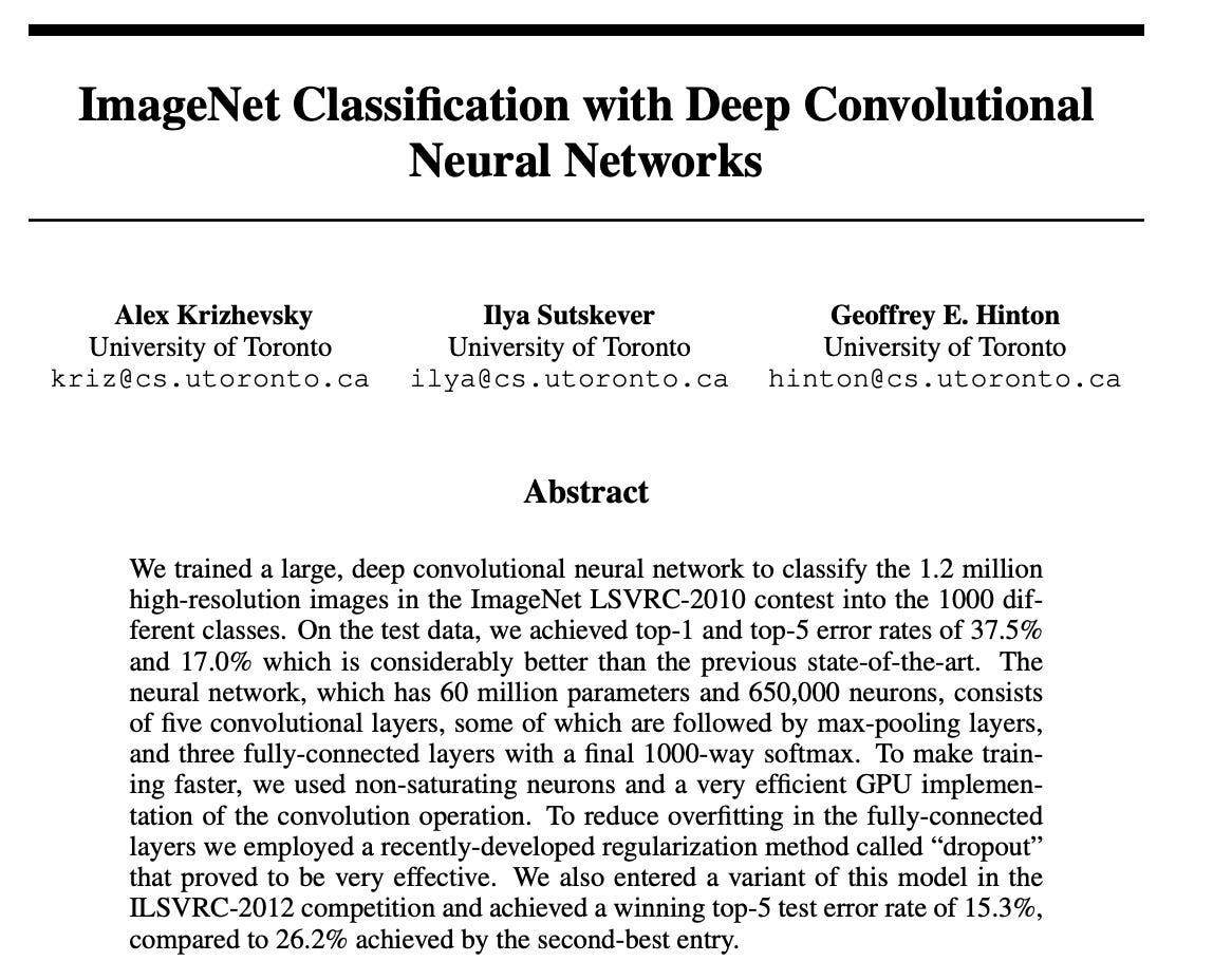
AlexNet: ImageNet Classification with Deep Convolutional Neural Networks
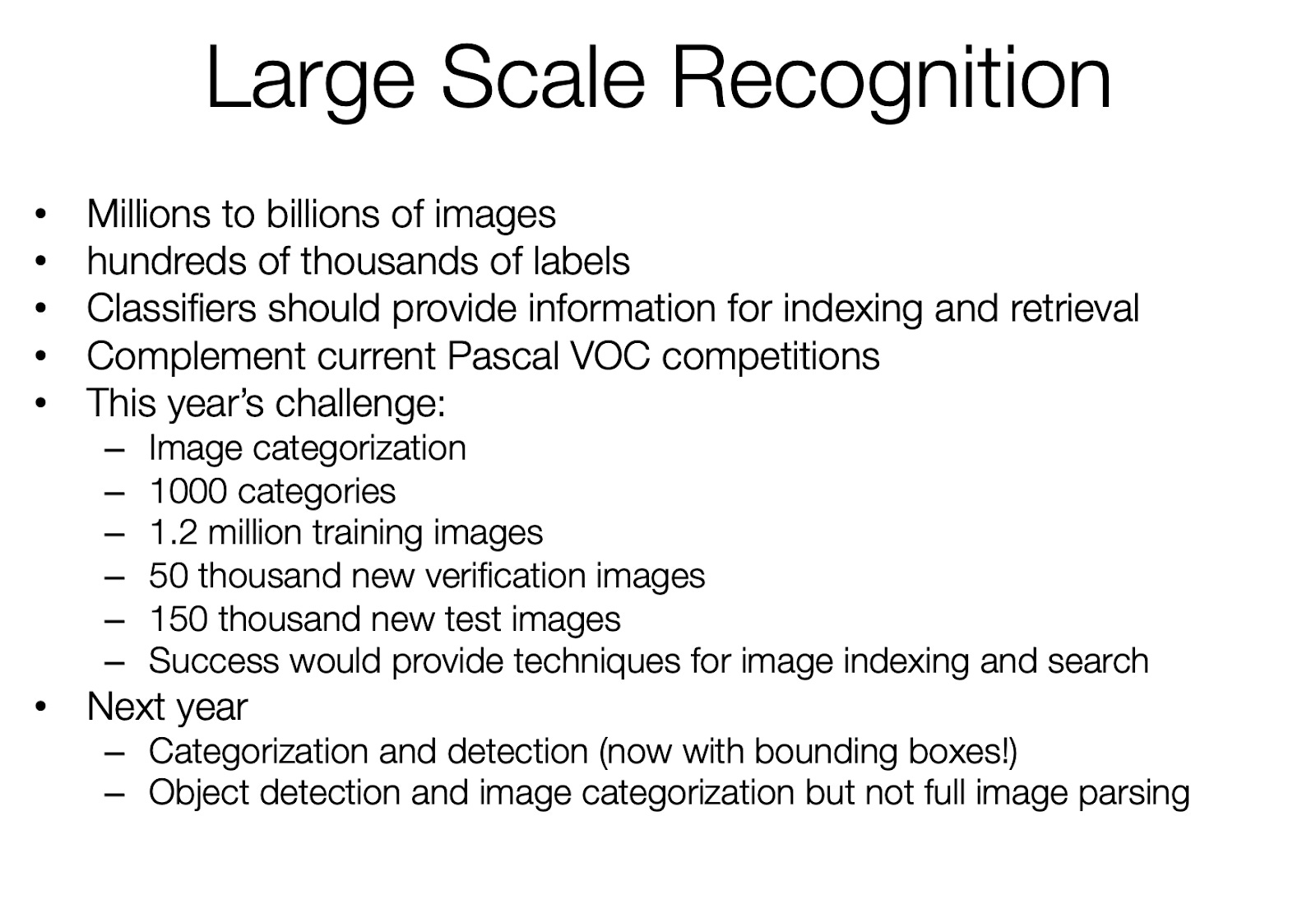
In 2010, a new computer vision competition was introduced where competitors used a subset of Li’s ImageNet database:
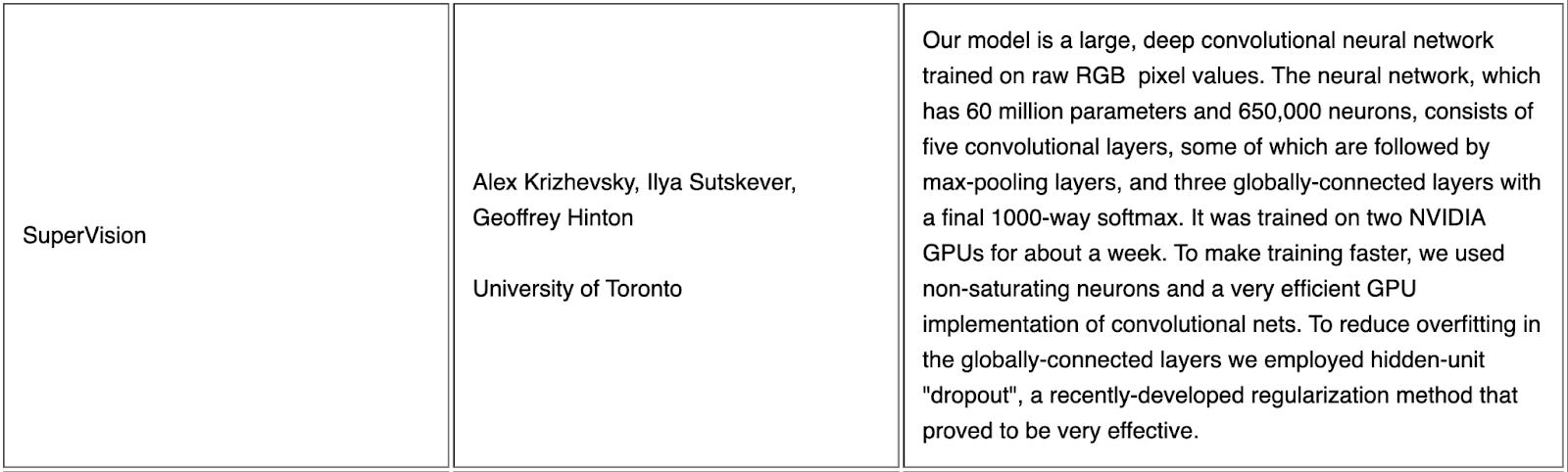
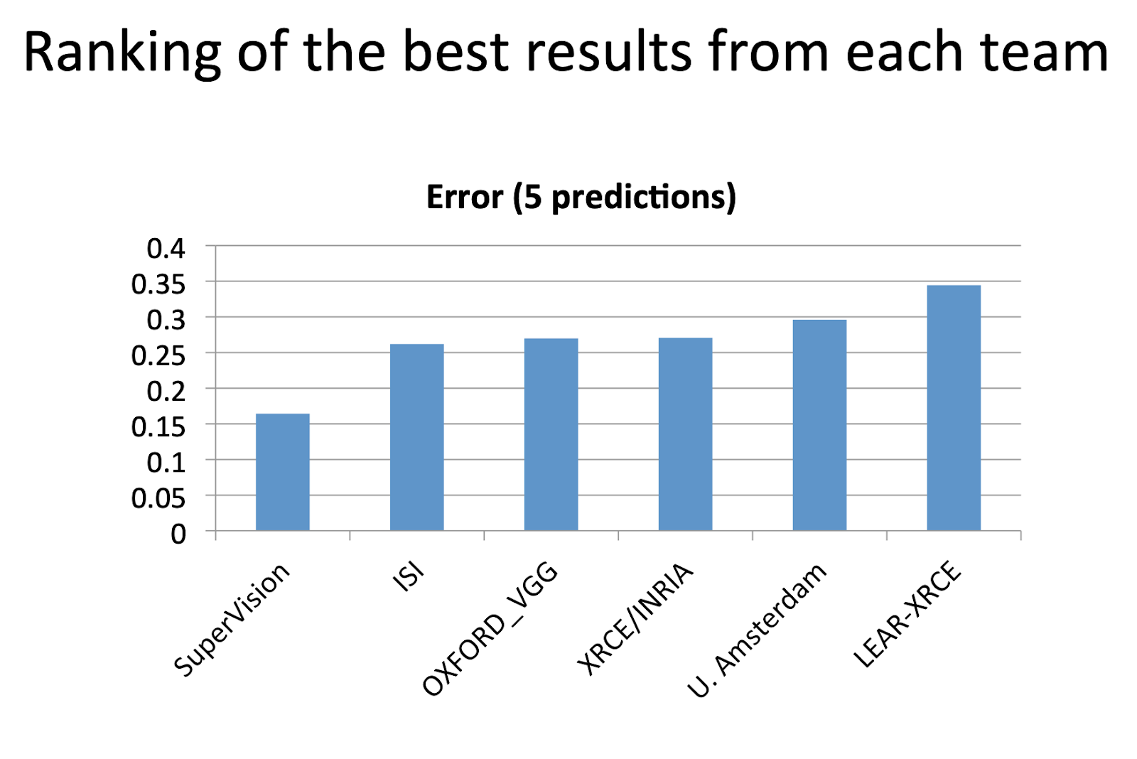
In 2012, team SuperVision from the University of Toronto entered the ImageNet competition with a deep convolutional neural network trained on two Nvidia GPUs.
Recognize any of these names? 😎
Team SuperVision’s neural net dominated the ImageNet 2012 competition:
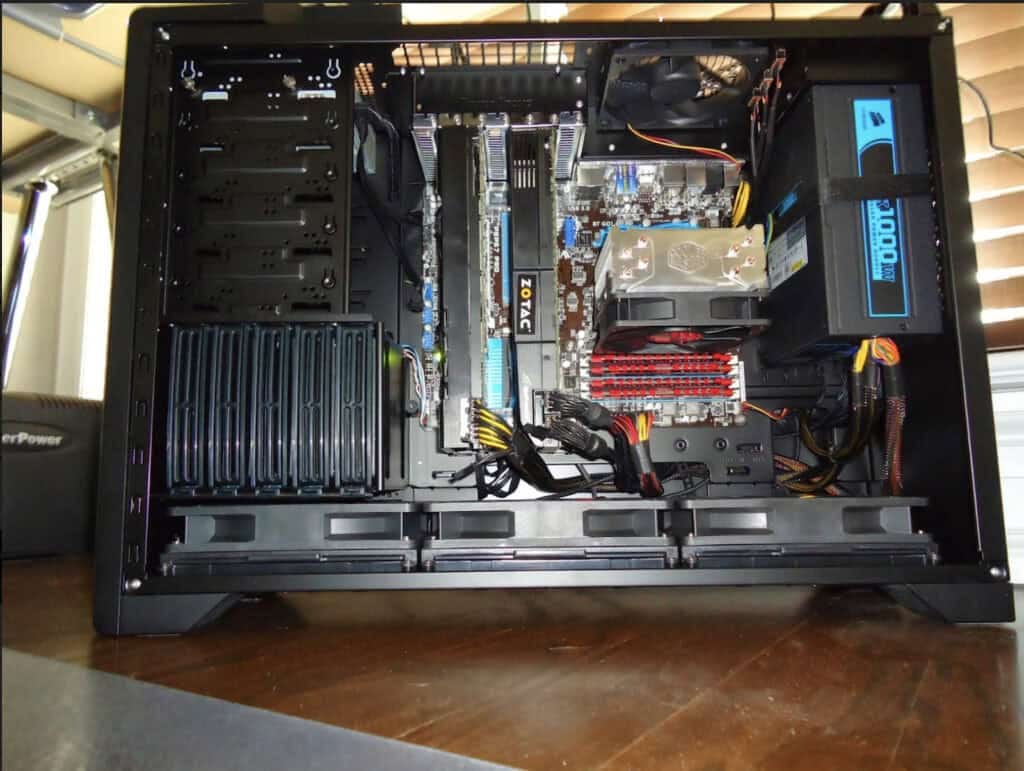
Sutskever convinced fellow Toronto graduate student Alex Krizhevsky, who had a keen ability to wring maximum performance out of GPUs, to train a convolutional neural network for ImageNet, with Hinton serving as principal investigator. Krizhevsky had already written CUDA code for a convolutional neural network using NVIDIA GPUs, called “cuda-convnet,” trained on the much smaller CIFAR-10 image dataset. He extended cuda-convnet with support for multiple GPUs and other features and retrained it on ImageNet. The training was done on a computer with two NVIDIA cards in Krizhevsky’s bedroom at his parents’ house. Over the course of the next year, Krizhevsky constantly tweaked the network’s parameters and retrained it until it achieved performance superior to its competitors. The network would ultimately be named AlexNet, after Krizhevsky.
In describing the AlexNet project, Geoff Hinton summarized for CHM: “Ilya thought we should do it, Alex made it work, and I got the Nobel Prize.”
The home computer with GPUs used to create AlexNet. Credit: University of Toronto via Computer History Museum website
Data + CUDA + 2 GPUs + 1 grad student = monumental change in computer vision history.
Remember the 1989 LeCun CNN with ~1000 neurons and ~70K weights? The 2012 AlexNet paper mentions 650,000 neurons and 60 million parameters!!!!
That’s the beauty of scaling computation (with parallel processing via GPUs) and data!
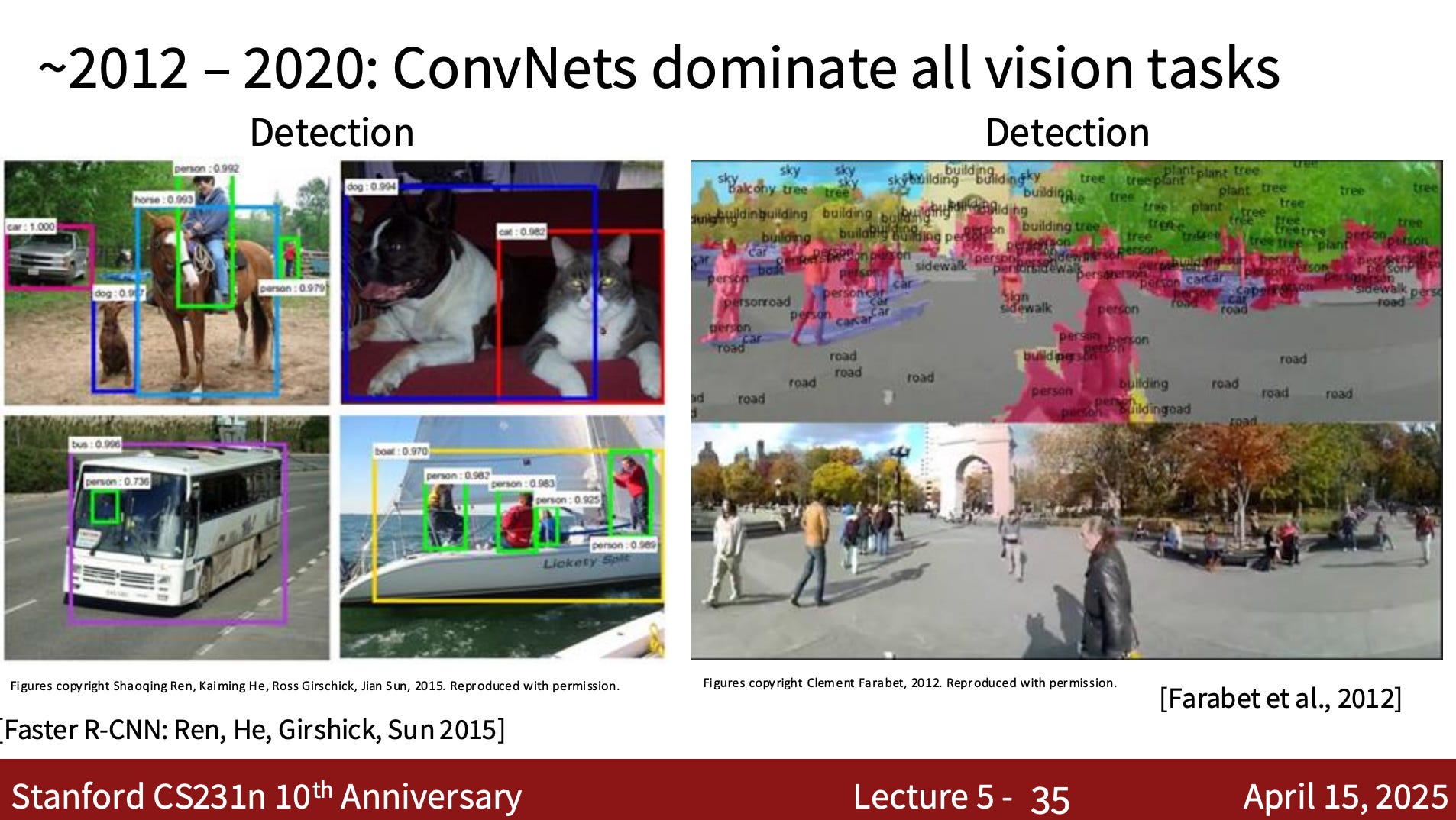
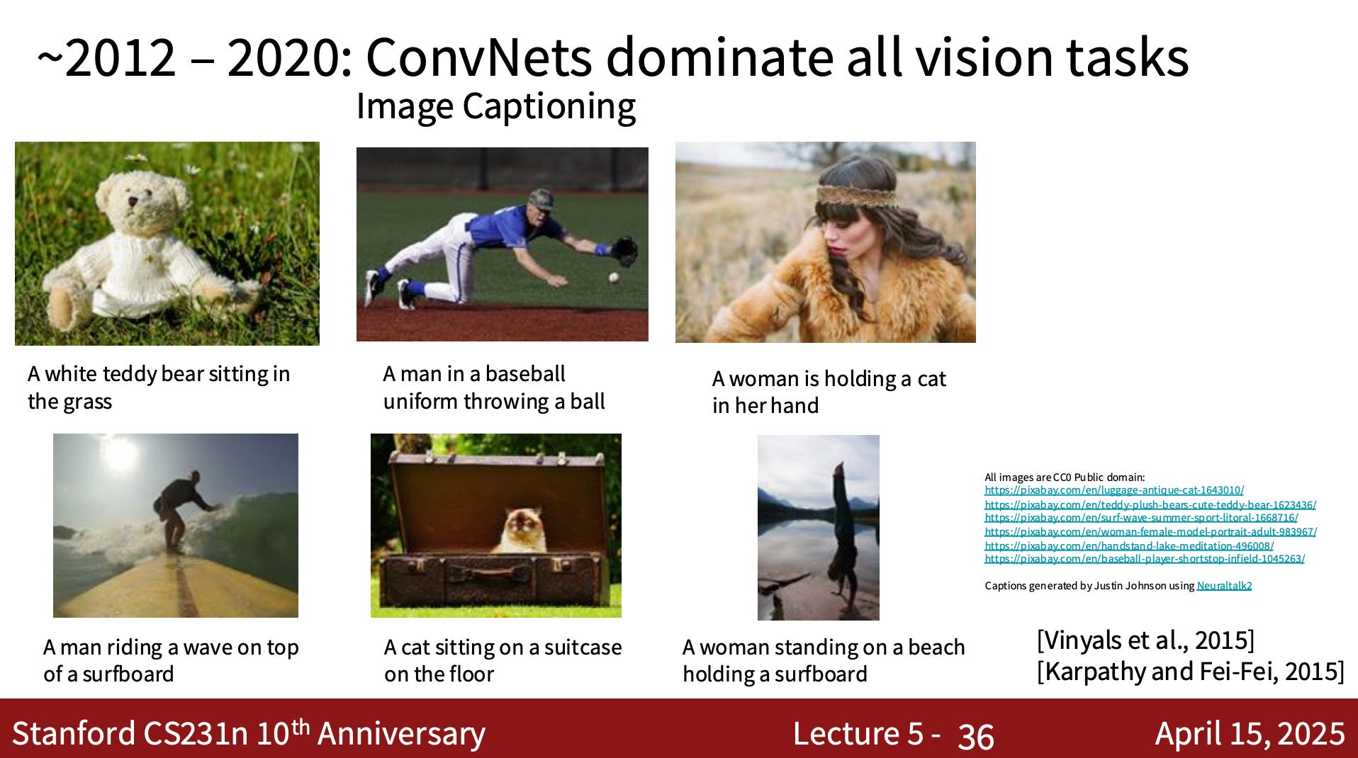
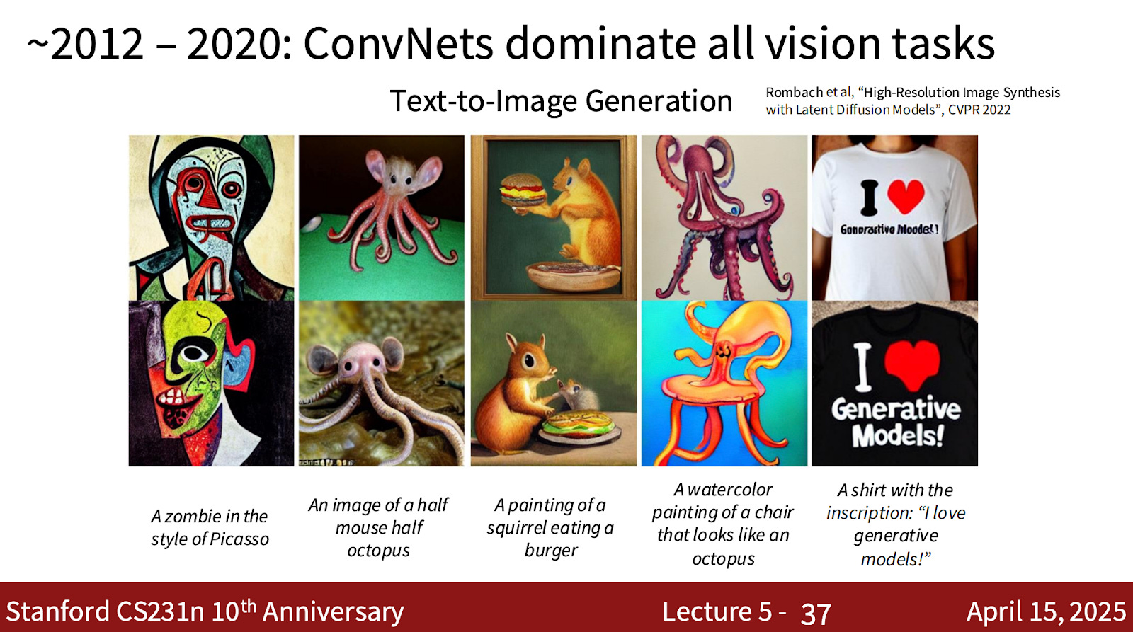
From 2012 onward, convolutional neural nets were the defining architecture for computer vision:
Could anything ever surpass the performance of ConvNets?
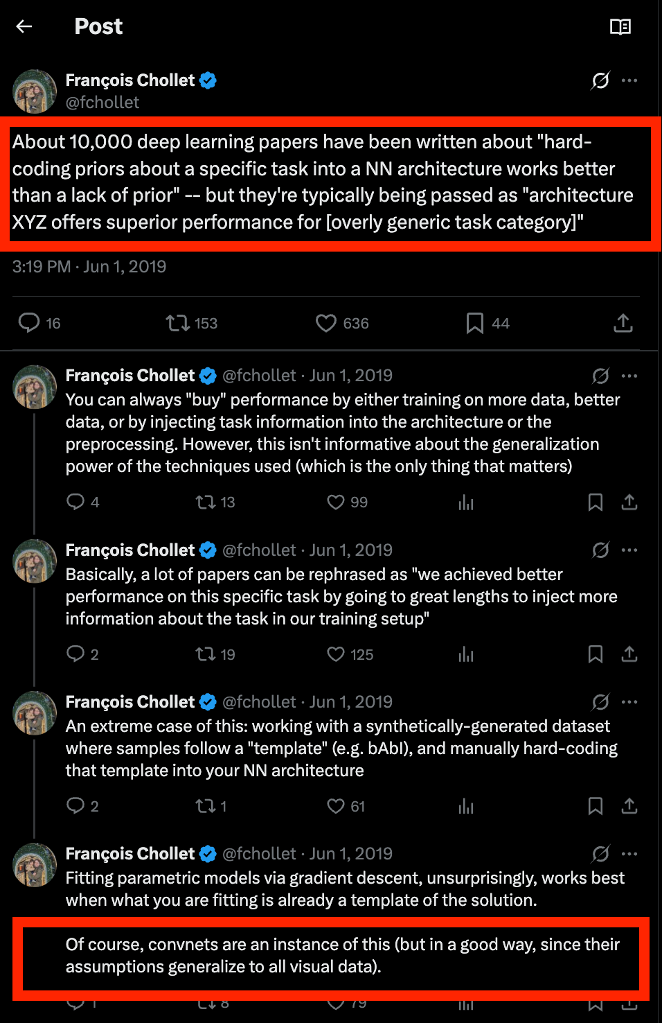
Here’s a hint from a 2019 François Chollet tweet:
Hmmmm…. convolutional neural networks hardcode priors into the neural network architecture…
Also in 2019, Richard Sutton posted his famous Bitter Lesson:
One thing that should be learned from the bitter lesson is the great power of general purpose methods, of methods that continue to scale with increased computation even as the available computation becomes very great. The two methods that seem to scale arbitrarily in this way are search and learning.
Could there be even more general methods that scale with more compute and more data and outperform ConvNets? On the one hand, ConvNets were already more general than other approaches, as Sutton mentioned in that Bitter Lesson post
In computer vision, there has been a similar pattern. Early methods conceived of vision as searching for edges, or generalized cylinders, or in terms of SIFT features. But today all this is discarded. Modern deep-learning neural networks use only the notions of convolution and certain kinds of invariances, and perform much better.
But… recall the 2017 introduction of a new neural network architecture, the Transformer, which does away with convolutions entirely:
We propose a new simple network architecture, the Transformer, based solely on attention mechanisms, dispensing with recurrence and convolutions entirely.
Maybe attention is all computer vision needs?
Well, that and a ton of data and computation scale.
Stay tuned for Part 2 😎
Chipstrat is a reader-supported publication. To receive new posts and support my work, consider becoming a free or paid subscriber.